SLAMBOOK Chapter5: Nonlinear Optimization

 

SLAMBOOK Chapter3: Lie Group and Lie Algebra

In SLAMBOOK Chapter3: Lie Group and Lie Algebra, we covered that the pose in the equation can be described by the transformation matrix and then optimized by Lie Algebra. Chapter5 provides a comprehensive exploration of why SLAM necessitates differentiation more extensively than chapter 3. The goal of chapter 5 is:

1. Understand the nonlinear optimization method
2. Learn how to use optimization libraries(Ceres / g2o)

State Estimation

$$ \left\{\begin{matrix}
x_{k} = f(x_{k-1},u_{k}) + w_{k} \\
z_{k,j} = h((y_{j},x_{k})) + v_{k,j}
\end{matrix}\right. $$

Recall that the \(x_{k}\) is the pose of the camera, which can be described by \(\mathbf{SE(3)}\), and \(z\) is the observation of the pinhole camera model. The reason for the need for optimization in SLAM is the inherent inaccuracy of sensors. The sensor data is corrupted by noise denoted by \(w_{k}, v_{k,j}\), and we make the assumption that the noise follows a Gaussian distribution.

$$ w_{k} \sim \mathcal{N}(0,R_{k}), v_{k} \sim \mathcal{N}(0,Q_{k,j}) $$

Under the influence of these noises, we hope to infer the pose \(x\) and the map \(y\) from the doisy data \(z\) and \(u\). 

In mathematical term, is to find the state \(x,y\) under the condition that the input data \(u\) and observation data \(z\):

$$ P(x,y| z,u) $$

To estimation the conditional pdf, we use the Bayes equation to switch the variables to easier form to solve:

Bayes theory

So the optimization in SLAM is now equivalent to solving:

$$ (x,y)^{*} = \mathrm{argmax}_{x,y}P(z,u|x,y) $$

 

Introduction to Least-squares

Since we assume the noise is Gaussian, the conditional probability of the obsevation data is:

 

$$ z_{j,k} = h(y_{j},x_{k}) + v_{k,j}, \quad v_{k} \sim \mathcal{N}(0,Q_{k,j}) \\ P(z_{j,k}|x_{k},y_{j}) = N(h(y_{j}, x_{k}), Q_{k,j})  $$

 

Taking the negative logarithm of a Gaussian distribution is commonly done in optimzation because it allows us to convert the problem of MLE(Maximize Likelihood Estimation) into a simpler form. 

$$ P(x) =\frac{1}{\sqrt{(2\pi)^N\det(\Sigma)}}\exp(-\frac{1}{2}(x-\mu)^T\Sigma^{-1}(x-\mu))  \\ -\ln {P(x)} =\frac{1}{2}\ln((2\pi)^N\det(\Sigma)) + \exp(-\frac{1}{2}(x-\mu)^T\Sigma^{-1}(x-\mu))$$

 

By minimizing the negative log-likelihood, we are essentially minimizing the discrepancy between the predicted mean and the observed data. Thus our SLAM optimization problem is equivalent to find such a solution:

$$ (x_{k}, y_{j})^{*} = \mathrm{argmax}\mathcal{N}(h(y_{j}, x_{k}), \mathbb{Q}_{k,j}) \\ = \mathrm{argmin}((z_{k,j} - h(x_{k},y_{j}))^{T} Q_{k,j}^{-1} ((z_{k,j} - h(x_{k},y_{j})) $$

 

For better understanding, let's look an example. Consider a very simple discrete-time system:

$$ \begin{matrix}
 x_{k} = x_{k-1}+u_{k} + w_{k}, \quad w_{k}\sim \mathcal{N}(0,Q_{k})\\ 
 z_{k} = x_{k} + n_{k}, \quad n_{k}\sim \mathcal{N}(0,R_{k})\\ k = 1,2,3
\end{matrix} $$

 

If we convert the optimization to a solvable least-square equation:

$$\mathrm{x}^{*} = \mathrm{argmax}P(\mathrm{x|u,z}) = \mathrm{argmax}P(\mathrm{u,z|x}) \\ = \prod_{k=1}^{3}P(u_{k}|x_{k-1},x_{k})\prod_{k=1}^{3}P(z_{k}|x_{k}) $$

let the error term between model and measurment as:

$$e_{u,k} = x_{k} - x_{k-1} - u_{k}, \quad e_{z,k} = z_{k} - x_{k} $$

then the least-square equation is:

$$ \sum_{k=1}^{3}e^{T}_{u,k}Q_{k}^{-1}e_{u,k} + \sum_{k=1}^{3}e^{T}_{z,k}R_{k}^{-1}e_{z,k}$$

For actual implementation to solve this system in a matrix form, define the vector \(\mathrm{y=[u,z]}^{T}\).

$$\mathrm{y - Hx = e}\sim \mathcal{N}(0,\Sigma) \\
\begin{bmatrix}
1 &-1  &0  & 0 \\
0 & 1 & -1 & 0 \\
0 & 0 &1  & -1 \\
0 & 1 & 0 & 0 \\
0 & 0 & 1 & 0 \\
0 & 0 & 0 & 1 \\
\end{bmatrix} $$

 

Nonlinear Least-square Problem

Newton-Rapson Method

With the assumption that models are linear, we can easily build and solve a linear system. However, most of the real-world environments are inherently nonlinear. Since SLAM involves nonlinear optimization techniques to iteratively refine the estimates of robot pose map, we need to know how to deal with the nonlinear least-square problems.

$$  \min_{x}F(x) = \frac{1}{2}\left\| f(x) \right\|_{2}^{2} $$

 

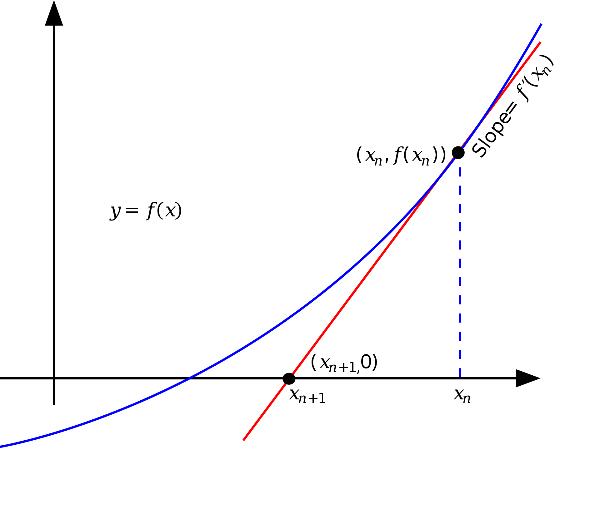
The Newton-Raphson method is commonly used for finding solution of a differentiable function. It is an iterative numerical method that can be used when it is difficult or impossible to find analytical soltuions for equation.

1. set to initial guess \(x_{0}\)
2. compute a better approximation by its tangent line \(x_{n+1} = x_{n} - \frac{f(x_{n})}{f^{'}(x_{n})} \).

The above example is the simplest form of single-variable scalar function \(\mathrm{R}\rightarrow \mathrm{R} \). If we extend to multi-variable function, parital derivative gradient denoted by \(\nabla \) is used as the tangent line. If the function is  \(\mathrm{R}^{n} \rightarrow \mathrm{R}^{m} \), Jacobian matrix \(J \)should be computed. 

 

Returning to the problem of minimizing the cost function, in order to minimize a general cost function \(F(\mathrm{x})\), the equation can be transformed into the problem of finding a solution for \(F'(\mathrm{x}) = 0\). According to the Taylor expansion of the cost function:

$$ F(\mathrm{x}_{k} + \Delta \mathrm{x}_{k}) \sim  F(\mathrm{x}_{k}) + \mathrm{J}(\mathrm{x}_{k})^{T} + \frac{1}{2}\Delta \mathrm{x}_{k}^{T}\mathrm{H}(\mathrm{x}_{k})\Delta \mathrm{x}_{k}$$

where \(\mathrm{J}, \mathrm{H}\) is the first and second-order derivative(Jacobian and Hessian). In each iteration, we can compute increment as:

$$ \Delta\mathrm{x}^{*} = \mathrm{argmin}(F(\mathrm{x}_{k} + \Delta \mathrm{x}_{k}) \sim  F(\mathrm{x}_{k}) + \mathrm{J}(\mathrm{x}_{k})^{T} + \frac{1}{2}\Delta \mathrm{x}_{k}^{T}\mathrm{H}(\mathrm{x}_{k})Delta \mathrm{x}_{k}) \\  \mathrm{J} + \mathrm{H}\Delta \mathrm{x} = 0 $$

 

However, the Newton's method needs to calculate the \(\mathrm{H}\) Hessian matrix, which is very time-expensive when the problem is large.

 

The Gauss-Newton Method

The Gauss-Newton method is used to solve nonlinear least square problems, which is equivalent to minimizing a sim of squared function values. Since we know the cost function is quadratic function of \(f(x)\)(Not \(F(x)\)), it is guaranteed that the cost function is convex.

$$ \Delta\mathrm{x}^{*} = \mathrm{argmin}(f(\mathrm{x}_{k} + \Delta \mathrm{x}_{k}) \sim  f(\mathrm{x}_{k}) + \mathrm{J}(\mathrm{x}_{k})^{T}\Delta \mathrm{x}_{k}) \\ \Delta\mathrm{x}^{*} = \mathrm{argmin} \frac{1}{2}\left\| f(x) + \mathrm{J(x)}^{T}\Delta \mathrm{x} \right\|^{2} $$

From the equation, the \(\Delta\mathrm{x}\) is obtained as:

$$ \mathrm{J(x)J}^{T}\mathrm{(x)}\Delta \mathrm{x} = -\mathrm{J(x)}f(\mathrm{x})$$

We call this optimzation method as Gauss-Newton optimization. 

 

There are also Levenberg-Marquardt method used for solving nonlinear least squareds problems. The difference is that the Levenberg-Marquardt method introduces a damping factor, which scales the contribution of the gradient descent update based on the current state of the optimization. It shares the same fundamental concept as Gauss-Newton, so